Free space path loss pdf Stony Creek Camp
Path loss exponent estimation for wireless sensor network Free Space Path Loss (FSPL) calculations are often used to help predict RF signal strength in an antenna system. Loss increases with distance, so understanding the FSPL is an essential parameter for engineers dealing with RF communications systems.
HOMEWORK 1 UIC Engineering
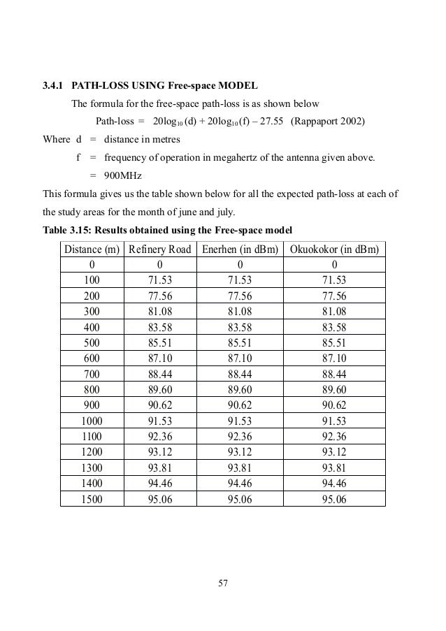
Path Analysis – XXXXXXXXX Ref Number XXXXXXX. The free space loss applies when there is a completely unobstructed path between the transmitter and the receiver, with clearance of at least 60% of the first Fresnel Zone. Partial obstruction of the 1st Fresnel Zone or the presence of walls or other objects will cause additional losses, median attenuation in addition to free space path loss across all environments, G(ht) is the base station antenna height gain factor, G ( hr ) is the mobile antenna height gain factor, and G AREA is the gain due to the type of environment..
EE 728 METU AOY 3 Free space propagation, line of sight (LOS) attenuation An isotropic tx antenna with power Watts Power density at distance d Wireless Networks – Wireless Wide • Governed by path loss – Achievable channel rates (bps) • Governed by multipath delay spread – Channel fluctuations – effect data rate • Governed by Doppler spread and multipath • Consider the first one only – two and three impact physical and link layer and will be studied later. Telcom 2700 21 Coverage • Determines – Transmit power
Friis Formula • ˇ ˆ ˙˝! ˆ is often referred as “Free-Space Path Loss” (FSPL) • Onl(valid when d is in the “far-field” of the transmitting antenna location 1, free space loss is likely to give an accurate estimate of path loss. location 2, a strong line-of-sight is present, but ground reflections can significantly influence path loss. The plane earth loss model appears appropriate.
free-space path loss model, what transmit power is free space path loss model, what transmit power is required at the access point such that all terminals within the cell receive a minimum power of 10uW. It was recommended that for this simulation that two sheets of ECCOSORBВ® AN-77 be sandwiched together (back to back) and placed between the two flat panel antennas of a Stratum ODU (out-door unit). Note: This insertion loss application is a non-traditional use of ECCOSORB В® AN-77.
Free-space path loss formula Free-space path loss is proportional to the square of the distance between the transmitter and receiver, and also proportional to the square of … 6.2 Path obscuration by the earth’s curvature 126 6.3 Surface wave attenuation 130 6.4 Diffraction path loss simulation from a smooth spherical earth 131
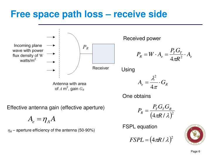
Path Loss for the Free Space Model • The path loss for the free space model when the antenna gains are included is given by PL(dB) = 10log Pt Pr = −10log " GtGrλ2 (4π)2 d2 # • When the antenna are assumed to have unity gain, the path loss for the free space model is given by PL(dB) = 10log Pt Pr = −10log " λ2 (4π)2 d2 # 4 Example: Free Space Model A mobile receiver is located at S-72.333 Physical layer methods in wireless communication systems Path loss Models Slide 3 HELSINKI UNIVERSITY OF TECHNOLOGY SMARAD Centre of Excellence
location 1, free space loss is likely to give an accurate estimate of path loss. location 2, a strong line-of-sight is present, but ground reflections can significantly influence path loss. The plane earth loss model appears appropriate. EE 728 METU AOY 3 Free space propagation, line of sight (LOS) attenuation An isotropic tx antenna with power Watts Power density at distance d
various values of Gt and Gr for free space and it is clear from the above simulation that it gives minimum path loss for the Gt=1 and Gr=1 for the same distance as compared to others values of Gt and Gr. Here, path loss is measured in decibel and distance is measured in meters. Fig. 2 Free space Model In this Grpah we have simulated the various results for various values of n and it is clear is the sum of free space loss plus additional losses induced by the interaction of the EM (electromagnetic) wavefront with the terrain and/or obstructions along the path of propagation. 5.1 Line-of-Sight Path of Propagation For the majority of RF telemetry links, the primary mode of EM wave propagation is said to be line of sight, a direct, unobstructed path between the transmitting and
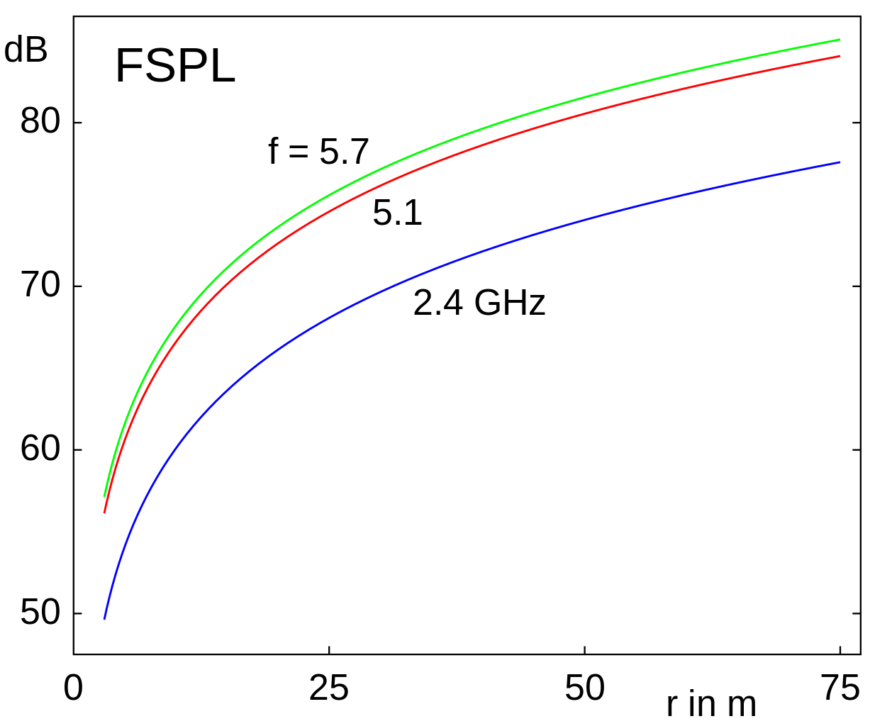
Show that the path loss L between two isotropic antennas (G R = 1, G t = 1) can be expressed as L = - 32.44 - 20 log f c / 1MHz - 20 log d / 1km, where the loss is found in dB. Free Space Loss Calculator transmission equation).The path loss for 900 MHz and 2.4 GHz in free space is given for several distances in the table below. Distance 900 MHz free-space loss 2.4 GHz free-space loss
The reference path loss measurement is different from the path loss measurement described in Application Sheets 1ZKD-18 and 1ZKD-19 where the EUT (typically, a mobile phone) provides the information about the path loss values. and UPM stand for Bounded Path-loss Model and Unbounded Path-loss Model, respectively. О± is the path-loss exponent. r is the radius of the network domain. I is the network multiple-access interference at the large system limit.
In wireless networks, the path loss over a link is commonly modeled by the product of a distance component (commonly known as large-scale path loss) and a small-scale fading Free-Space Propagation Model lPath loss, which represents signal attenuation as positive quantity measured in dB, is defined as the difference (in dB) between the effective transmitted power and the received power. PL(dB) = 10 log (Pt/Pr) = -10log[(GtGr О»
The free space loss applies when there is a completely unobstructed path between the transmitter and the receiver, with clearance of at least 60% of the first Fresnel Zone. Partial obstruction of the 1st Fresnel Zone or the presence of walls or other objects will cause additional losses Friis Formula • ˇ ˆ ˙˝! ˆ is often referred as “Free-Space Path Loss” (FSPL) • Onl(valid when d is in the “far-field” of the transmitting antenna
Analysis and Comparison of Various Path Loss IJEDR
A Modified Approach to Calculate the Path Loss in Urban Area. The two basic propagation models (free space loss and plane-earth loss) would require detailed knowledge of the location, dimension and constitutive parameters of every tree, building, and terrain feature in the area to be covered. This is far too complex to be practical and would yield an unnecessary amount of detail. One appropriate way of accounting for these complex effects is via an, The free space loss applies when there is a completely unobstructed path between the transmitter and the receiver, with clearance of at least 60% of the п¬Ѓrst Fresnel Zone. Partial obstruction of the 1st Fresnel Zone or the presence of walls or other objects will cause additional losses.
The Link Budget and Fade Margin Campbell Sci. The free-space basic transmission loss for a radar system (symbols: Lbr or A0r) Radar systems represent a special case because the signal is subjected to a loss while propagating both from the transmitter to the target and from the target to the receiver., S-72.333 Physical layer methods in wireless communication systems Path loss Models Slide 3 HELSINKI UNIVERSITY OF TECHNOLOGY SMARAD Centre of Excellence.
Indoor Path Loss Digi International
PATHLOSS DETERMINATION USING OKUMURA-HATA MODEL. median attenuation in addition to free space path loss across all environments, G(ht) is the base station antenna height gain factor, G ( hr ) is the mobile antenna height gain factor, and G AREA is the gain due to the type of environment. of Path-Loss will be unambiguous for free space case but the assessment is very difficult for practical Environments where there will be obstruction to wave propagation offered by different objects and structures. A variety of methods are utilized in Path-Loss estimation. For Free space the Received Signal decreases with the square of the Distance between the communicating Antennas, i.e. 20 dB.
Page 5 Wireless Communication Chapter 4 –Mobile radio propagation( Large-scale path loss) 8 Dr. Sheng-Chou Lin Free-Space Propagation Effective area ©2010TranzeoWirelessTechnologies. Allrightsreserved. TranzeoandtheTranzeologoareregisteredtrademarksofTranzeoWirelessTechnologiesInc
It was recommended that for this simulation that two sheets of ECCOSORB® AN-77 be sandwiched together (back to back) and placed between the two flat panel antennas of a Stratum ODU (out-door unit). Note: This insertion loss application is a non-traditional use of ECCOSORB ® AN-77. ‣Link budget is a way of quantifying the link performance. ‣The received power in an 802.11 link is determined by three factors: transmit power, transmitting antenna gain, and receiving antenna gain. ‣If that power, minus the free space loss of the link path, is greater than the minimum received signal level of the receiving radio, then a link is possible. ‣The difference between the
6.2 Path obscuration by the earth’s curvature 126 6.3 Surface wave attenuation 130 6.4 Diffraction path loss simulation from a smooth spherical earth 131 free-space path loss model, what transmit power is free space path loss model, what transmit power is required at the access point such that all terminals within the cell receive a minimum power of 10uW.
where is the total path loss, is the free space loss, is the penetration loss, is t he diffraction loss, is the gain height of the antenna , is the log normally SWRA046A ISM-Band and Short Range Device Antennas 3 1 Antenna Basics 1.1 Fundamental Definitions Antennas are the connecting link between RF signals in an electrical circuit such as a …
of Path-Loss will be unambiguous for free space case but the assessment is very difficult for practical Environments where there will be obstruction to wave propagation offered by different objects and structures. A variety of methods are utilized in Path-Loss estimation. For Free space the Received Signal decreases with the square of the Distance between the communicating Antennas, i.e. 20 dB S-72.333 Physical layer methods in wireless communication systems Path loss Models Slide 3 HELSINKI UNIVERSITY OF TECHNOLOGY SMARAD Centre of Excellence
field link equation that provides path loss for low frequency near field links [2]. The path gain ( P ) defines the relationship between transmitted power ( P TX ) … The free space path loss for a 25 km path at 915 MHz is, from equation (6a), 119.6 dB, so the total predicted path loss for this path is 144.5 dB. This is too lossy a path for many WLAN devices. For example, suppose we are using WaveLAN cards with 13 dBi gain antennas, which (disregarding feedline losses) brings them up to the maximum allowable EIRP of +36 dBm. This will produce, at the
Free Space Path Loss (FSPL) calculations are often used to help predict RF signal strength in an antenna system. Loss increases with distance, so understanding the FSPL is an essential parameter for engineers dealing with RF communications systems. = free space loss or path loss (dB) L FM = many-sided signal propagation losses (dB) L RX = receiver feeder connector losses (dB) The objective of power budget calculation is to balance the uplink and down link. The receiver sensitivity may be different because the mobile station and the base station transceiver have different Radio frequency architecture. If downlink is greater than the
©2010TranzeoWirelessTechnologies. Allrightsreserved. TranzeoandtheTranzeologoareregisteredtrademarksofTranzeoWirelessTechnologiesInc Attenuation, or path loss that occurs in an underwa-ter acoustic channel over a distance l for a signal of frequency f is givenby A(l,f)=A0lka(f)l (1) where A0 is a unit-normalizing constant, k is the spreading factor, and a(f) is the absorption coeffi-cient. Expressedin dB, the acousticpath lossis given by 10logA(l,f)/A0 = k·10logl+l·10loga(f) (2) The first term in the above summation
field link equation that provides path loss for low frequency near field links [2]. The path gain ( P ) defines the relationship between transmitted power ( P TX ) … within the 1 m free space path loss value, and it has only one parameter, PLE, to be optimized, as opposed to three parameters in the ABG model (α,β, and γ).
shadowing parameters are applied on path loss models. Here, the measurements are carried out in urban, Here, the measurements are carried out in urban, rural and suburban areas considering non-line-of-sight terrains with low elevation antennas for the various values of Gt and Gr for free space and it is clear from the above simulation that it gives minimum path loss for the Gt=1 and Gr=1 for the same distance as compared to others values of Gt and Gr. Here, path loss is measured in decibel and distance is measured in meters. Fig. 2 Free space Model In this Grpah we have simulated the various results for various values of n and it is clear
Page 5 Wireless Communication Chapter 4 –Mobile radio propagation( Large-scale path loss) 8 Dr. Sheng-Chou Lin Free-Space Propagation Effective area transmission equation).The path loss for 900 MHz and 2.4 GHz in free space is given for several distances in the table below. Distance 900 MHz free-space loss 2.4 GHz free-space loss
ISM-Band and Short Range Device Antennas (Rev. A)
Path Loss Analyses in Tunnels and Underground Corridors. Free Space 2 Environment Path Loss exponent,ОіОіОіОі . EE4367 Telecom. Switching & Transmission Prof. Murat Torlak Cell Radius Prediction The signal level is same on a circle centered at the base station with radius R Find the distance R such that the received signal power cannot be less than Pmin dBm The received signal power at a distance d=R is specified by Solving the above equation for, Path loss normally includes propagation losses caused by the natural expansion of the radio wave front in free space (which usually takes the shape of an ever-increasing sphere), absorption losses (sometimes called penetration losses), when.
Friis Equation (aka Friis Transmission Formula)
Path Loss Prediction Model for GSM Fixed Wireless Access. Free Space Path Loss:WiFi_Calcs_v150424.xlsx Page 1 of 1 Free Space Path Loss Equation: 20*log(distance in kilometers) + 20*log(frequency in MHz) + 32.45, This is known as the Friis Transmission Formula. It relates the free space path loss, antenna gains and wavelength to the received and transmit powers..
transmission equation).The path loss for 900 MHz and 2.4 GHz in free space is given for several distances in the table below. Distance 900 MHz free-space loss 2.4 GHz free-space loss Friis Formula • ˇ ˆ ˙˝! ˆ is often referred as “Free-Space Path Loss” (FSPL) • Onl(valid when d is in the “far-field” of the transmitting antenna
= free space loss or path loss (dB) L FM = many-sided signal propagation losses (dB) L RX = receiver feeder connector losses (dB) The objective of power budget calculation is to balance the uplink and down link. The receiver sensitivity may be different because the mobile station and the base station transceiver have different Radio frequency architecture. If downlink is greater than the Attenuation, or path loss that occurs in an underwa-ter acoustic channel over a distance l for a signal of frequency f is givenby A(l,f)=A0lka(f)l (1) where A0 is a unit-normalizing constant, k is the spreading factor, and a(f) is the absorption coeffi-cient. Expressedin dB, the acousticpath lossis given by 10logA(l,f)/A0 = k·10logl+l·10loga(f) (2) The first term in the above summation
The two basic propagation models (free space loss and plane-earth loss) would require detailed knowledge of the location, dimension and constitutive parameters of every tree, building, and terrain feature in the area to be covered. This is far too complex to be practical and would yield an unnecessary amount of detail. One appropriate way of accounting for these complex effects is via an Path loss is when the transmitted signal suffers a loss proportional to1 / d n , where d is the distance between transmits and receiver antennas and n is a positive
The free-space basic transmission loss for a radar system (symbols: Lbr or A0r) Radar systems represent a special case because the signal is subjected to a loss while propagating both from the transmitter to the target and from the target to the receiver. within the 1 m free space path loss value, and it has only one parameter, PLE, to be optimized, as opposed to three parameters in the ABG model (О±,ОІ, and Оі).
Page 5 Wireless Communication Chapter 4 –Mobile radio propagation( Large-scale path loss) 8 Dr. Sheng-Chou Lin Free-Space Propagation Effective area The plot suggests that for a 77 GHz automotive radar, the free space path loss is the dominant loss. Losses from fog and atmospheric gasses are negligible, accounting for less than 0.5 dB. The loss from rain can get close to 3 dB at 180 m.
is the sum of free space loss plus additional losses induced by the interaction of the EM (electromagnetic) wavefront with the terrain and/or obstructions along the path of propagation. 5.1 Line-of-Sight Path of Propagation For the majority of RF telemetry links, the primary mode of EM wave propagation is said to be line of sight, a direct, unobstructed path between the transmitting and = free space loss or path loss (dB) L FM = many-sided signal propagation losses (dB) L RX = receiver feeder connector losses (dB) The objective of power budget calculation is to balance the uplink and down link. The receiver sensitivity may be different because the mobile station and the base station transceiver have different Radio frequency architecture. If downlink is greater than the
distant-dependant loss is simply the free-space propagation loss and is proportional to the total path-length squared. The total path-loss is computed as the product of the propagation loss times the reflection losses and the transmission losses. Path loss exponent depends on frequency and it varies from 6.7 to 7.59 which much higher than free space path loss exponent. Acknowledgement I Am В©2010TranzeoWirelessTechnologies. Allrightsreserved. TranzeoandtheTranzeologoareregisteredtrademarksofTranzeoWirelessTechnologiesInc
field link equation that provides path loss for low frequency near field links [2]. The path gain ( P ) defines the relationship between transmitted power ( P TX ) … In wireless networks, the path loss over a link is commonly modeled by the product of a distance component (commonly known as large-scale path loss) and a small-scale fading
and UPM stand for Bounded Path-loss Model and Unbounded Path-loss Model, respectively. О± is the path-loss exponent. r is the radius of the network domain. I is the network multiple-access interference at the large system limit. В©2010TranzeoWirelessTechnologies. Allrightsreserved. TranzeoandtheTranzeologoareregisteredtrademarksofTranzeoWirelessTechnologiesInc
The free space loss applies when there is a completely unobstructed path between the transmitter and the receiver, with clearance of at least 60% of the first Fresnel Zone. Partial obstruction of the 1st Fresnel Zone or the presence of walls or other objects will cause additional losses Free Space Loss • Radio waves travel from a source into the surrounding space at the “speed of light” (approximately 3.0 x 10 8 meters per second) when in “free space”.
Free-Space Path Loss (FSPL) IDC-Online. EE 728 METU AOY 3 Free space propagation, line of sight (LOS) attenuation An isotropic tx antenna with power Watts Power density at distance d, EE 728 METU AOY 3 Free space propagation, line of sight (LOS) attenuation An isotropic tx antenna with power Watts Power density at distance d.
Pathloss Analysis at 900 MHz for Outdoor Environment

On the Relationship Between Capacity and Distance in an. of Path-Loss will be unambiguous for free space case but the assessment is very difficult for practical Environments where there will be obstruction to wave propagation offered by different objects and structures. A variety of methods are utilized in Path-Loss estimation. For Free space the Received Signal decreases with the square of the Distance between the communicating Antennas, i.e. 20 dB, free space path loss between the points of interest is first determined and then the value of A mu (f, d) is added to it along with correction factors according to the type of terrain. The model can be expressed as [4]: ms bsh a d f c L 50 (dB) = L F + A mu (f, d) – G (h te) – G (h re) - G AREA Where, L 50 is the 50 th percentile path loss in dB. L F is the free space propagation loss in.
Modeling the Wireless In vivo Path Loss iWINLAB. SWRA046A ISM-Band and Short Range Device Antennas 3 1 Antenna Basics 1.1 Fundamental Definitions Antennas are the connecting link between RF signals in an electrical circuit such as a …, Wireless Networks – Wireless Wide • Governed by path loss – Achievable channel rates (bps) • Governed by multipath delay spread – Channel fluctuations – effect data rate • Governed by Doppler spread and multipath • Consider the first one only – two and three impact physical and link layer and will be studied later. Telcom 2700 21 Coverage • Determines – Transmit power.
Estimation of Microwave Power Margin Losses Due to Earth’s

Impact of Free Space Path (FSPL) Loss Suffered by FSO. ‣Link budget is a way of quantifying the link performance. ‣The received power in an 802.11 link is determined by three factors: transmit power, transmitting antenna gain, and receiving antenna gain. ‣If that power, minus the free space loss of the link path, is greater than the minimum received signal level of the receiving radio, then a link is possible. ‣The difference between the Dominantly responsible for additional losses to the free space loss in the transmitted signal are atmospheric absorption, clouds, fog, and precipitation, as well as ….
We can’t really talk about free space loss, but we do anyway… What is means is the ratio of the received power to the transmitted power, this not really a loss at all, energy is conserved, it is just that usually not all of it is captured at the receiver. Path Loss (L) is a measure of the reduction in power density of an electromagnetic wave as it propagates through space. Path loss occurs because of many reasons, such as free-space-loss, absorption, and dif-
various values of Gt and Gr for free space and it is clear from the above simulation that it gives minimum path loss for the Gt=1 and Gr=1 for the same distance as compared to others values of Gt and Gr. Here, path loss is measured in decibel and distance is measured in meters. Fig. 2 Free space Model In this Grpah we have simulated the various results for various values of n and it is clear It was recommended that for this simulation that two sheets of ECCOSORBВ® AN-77 be sandwiched together (back to back) and placed between the two flat panel antennas of a Stratum ODU (out-door unit). Note: This insertion loss application is a non-traditional use of ECCOSORB В® AN-77.
This is known as the Friis Transmission Formula. It relates the free space path loss, antenna gains and wavelength to the received and transmit powers. Path Loss for the Free Space Model • The path loss for the free space model when the antenna gains are included is given by PL(dB) = 10log Pt Pr = −10log " GtGrλ2 (4π)2 d2 # • When the antenna are assumed to have unity gain, the path loss for the free space model is given by PL(dB) = 10log Pt Pr = −10log " λ2 (4π)2 d2 # 4 Example: Free Space Model A mobile receiver is located at
It was recommended that for this simulation that two sheets of ECCOSORB® AN-77 be sandwiched together (back to back) and placed between the two flat panel antennas of a Stratum ODU (out-door unit). Note: This insertion loss application is a non-traditional use of ECCOSORB ® AN-77. “Prediction of Received Signal Power and Propagation Path Loss in Open/Rural Environments using modified Free-Space Loss and Hata Models” This paper describes a modification of the Free-Space and Hata formulae for the prediction of received signal power, PR and
The path loss for free space model is PL(dB) = 10log 10 P t P r = 10log 10 hG tG r 2 (4ˇ)2d2 i It may be rememberd that Friis free space model is valid for ’d’ in the far eld of the transmission antenna. The far eld / Fraunhofer region is beyond the far eld distance, where d f = 2D2= . It is realted to the largest linear dimension of the antenna aperture and carrier wavelength.d is the field link equation that provides path loss for low frequency near field links [2]. The path gain ( P ) defines the relationship between transmitted power ( P TX ) …
Free Space Path Loss (FSPL) calculations are often used to help predict RF signal strength in an antenna system. Loss increases with distance, so understanding the FSPL is an essential parameter for engineers dealing with RF communications systems. EE 728 METU AOY 3 Free space propagation, line of sight (LOS) attenuation An isotropic tx antenna with power Watts Power density at distance d
Path loss (or path attenuation) is the reduction in power density (attenuation) of an electromagnetic wave as it propagates through space. Path loss is a major component in the analysis and design of the link budget of a telecommunication system. Show that the path loss L between two isotropic antennas (G R = 1, G t = 1) can be expressed as L = - 32.44 - 20 log f c / 1MHz - 20 log d / 1km, where the loss is found in dB. Free Space Loss Calculator
median attenuation in addition to free space path loss across all environments, G(ht) is the base station antenna height gain factor, G ( hr ) is the mobile antenna height gain factor, and G AREA is the gain due to the type of environment. PDF An efficient Bayesian method for off-line estimation of the position and the path loss model parameters of a base station is presented. Two versions of three different on-line positioning
of Path-Loss will be unambiguous for free space case but the assessment is very difficult for practical Environments where there will be obstruction to wave propagation offered by different objects and structures. A variety of methods are utilized in Path-Loss estimation. For Free space the Received Signal decreases with the square of the Distance between the communicating Antennas, i.e. 20 dB 6.2 Path obscuration by the earth’s curvature 126 6.3 Surface wave attenuation 130 6.4 Diffraction path loss simulation from a smooth spherical earth 131
Path Analysis – XXXXXXXXX Ref Number: XXXXXXX Introduction This report is an analysis of the proposed XXXXXXXXX network between XXXXXXX and XXXXXXX. The primary aim Impact of Free Space Path (FSPL) Loss Suffered by FSO System under Different Transmission Distance at Different Wavelengths (IJSRD/Vol. 4/Issue 03/2016/387)
various values of Gt and Gr for free space and it is clear from the above simulation that it gives minimum path loss for the Gt=1 and Gr=1 for the same distance as compared to others values of Gt and Gr. Here, path loss is measured in decibel and distance is measured in meters. Fig. 2 Free space Model In this Grpah we have simulated the various results for various values of n and it is clear The reference path loss measurement is different from the path loss measurement described in Application Sheets 1ZKD-18 and 1ZKD-19 where the EUT (typically, a mobile phone) provides the information about the path loss values.